Mungebits
Machine learning appears at first glance to be the science of devising and answering pure statistical questions on real-life data sets. In practice, a lot of it ends up being data janitor work.
Turning the data cleaning and feature engineering process into a quick workflow and as pleasant a task as trying out different modeling methodologies will eventually address this problem.
Since parsing and merging of data is not typically R's forte let's restrict the discussion to transforming one messy, raw dataset into a clean, ready-to-model dataset before proceeding with more complicated modeling topologies.
The initial abstraction offered by the Syberia modeling engine is that of mungebits: atomic production-ready feature engineering templates that can be used to quickly clean a dataset without having to write separate code when it comes time to replicate the cleaning process on single rows of data.
Why would we want to replicate the entire process? That's precisely one of the difficulties that emerges when it comes time to "productionize" the model! The trained classifier expects a certain type of covariate matrix, namely the one in exactly the preprocessed format you generated by cleaning the data set.
But why would we want to think about "productionizing" right away when we are experimenting? Because if we don't, we will spend weeks or months on the long, error-prone translation process of turning an experimental result into one that can be applied on new data in the real world.
It's worth investing a little bit more time now instead of far more time later when we have to replicate the cleaning work on new data. Note this does not just apply to streaming systems! If someone gave you a new validation set from their data warehouse and asked to verify the performance on some new data points it would be equivalent to solving the streaming problem: we would have to replicate the entire cleaning process on the raw validation set.
For example, if you replaced messed up values with the correct values, imputed missing values, dropped certain columns, or derived some new features from the existing data, you will have to re-do that work when a single data point comes in--otherwise the trained classifier will be confused.
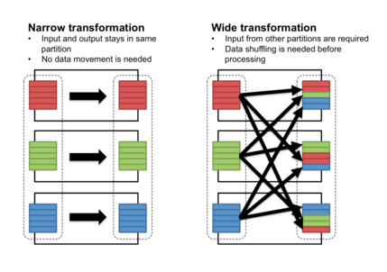
Operations that take one data.frame
and return another data.frame come
in two types: narrow and wide transformations. You can
delegate the narrow transformations to an ETL engineer or other
data curation role. However, this might not be feasible if we are deploying
a model, because they will have to provide a way to replicate their
process in real-time as well, for example through an API.
Narrow transformations, operations that can be done row-by-row without looking at the other rows, almost by definition do not need to store metadata to be reproduced on a single row. However, many of the most useful cleaning operations on a dataset—like sure independence screening, principal component analysis, imputation, discretization, aggregation and computation of ratios, numericalization of categorical features, and so on—are wide transformations.
The abundance of useful wide transformations is the reason why feature engineering cannot be separated from statistical modeling. It is impossible to have one person's role be maintaining a data pipeline while another person independently maintains a statistical model without running into a messy combinatorial explosion: they are inseparable aspects of the same task, in the same way database operations cannot be separated from a web application but instead compose its heart.
Let's convince ourselves that this is true.
The Basic Mungebit
Every time you write a script that begins with read.csv("data.csv")
and ends with a clean data set you have actually produced an
endomorphism on the space of dataframes, that is, a function
which takes one dataframe and yields another dataframe. Functions that
have the same domain and co-domain are really cool because they can
be trivially composed: if I have several such functions, I can just
apply them one after the other without worrying about setting up a complex
input/output graph since I know the input and the result will always be
a dataframe. (For the mathematically inclined, endomorphisms of any space form
a monoid under composition.)
In algebra class we were able to prove beautiful facts about parabolas and
the other conic sections because we looked at the most general cases, like
y = a * x^2 + b * x + c. Here, a,
b, and c are parameters:
for any combination of such three constants drawn from the real numbers we
get a different parabola.
Parametrization is powerful because it means we don't have to repeat our work every time a special case comes along. Finding the quadratic equation can be done once; the other times we simply plug in the parameters! Every time you write the type of code below you are re-deriving the quadratic formula by hand.
# Uncomment the line below if you want to run this on an example.
# raw_data <- data.frame(occupation = c("Doctor", rep("Waiter", 200)), stringsAsFactors = FALSE)
raw_data$occupation <- ave(raw_data$occupation, raw_data$occupation, FUN = function(x) {
  if (length(x) / NROW(raw_data) < 0.01) { # Percentage of population with this occupation.
    "Other"
  } else {
    x[1L]
  }
})
If we later decide to perform the same operation on another variable, the path of lowest resistance will be copying the above and replacing "occupation" with the other variable name. If instead we had parametrized this as a function that took a dataset, the variables to alter, and a minimal threshold for replacing the value with "Other," we could easily re-use it for a variety of datasets.
What about when it comes time to replay the operation on a single row of data or a new validation set? The above code won't run! With a single row of data, all values will always have trivially 100% incidence and nothing will ever be replaced with "Other," which might lead to unexpected results when it comes to our classifier. Now imagine this problem amplified by 100 more feature engineering steps on a dataset with 1000s of variables. This is why data cleaning is seen as a combinatorial nightmare.
But it does not have to be. Mungebits solve this problem, and a proper generalization of mungebits solves any problem of taking raw, messy data sets, joining and munging them until there's a clean covariate matrix on which we can train a model—without having to ever write a custom data pipeline, instead making the process part of the explorative data science journey.
So what does a mungebit for the above step look like?
# lib/mungebits/remove_uncommon_values.R
train <- function(dataframe, variables, threshold = 0.01, replacement = "Other") {
  replacements <- list()
  for (v in variables) {
    dataframe[[v]] <- ave(dataframe[[v]], dataframe[[v]], FUN = function(x) {
      if (length(x) / NROW(dataframe) < threshold) {
        replacements[[v]] <<- c(replacements[[v]], x[1L])
        "Other"
      } else {
        x[1L]
      }
    })
  }
  # We'll learn about the "input" helper shown below later on.
  input$replacements <- replacements
  dataframe
}

predict <- function(dataframe, variables, threshold = 0.01, replacement = "Other") {
  variables <- intersect(colnames(dataframe), variables)
  for (v in names(input$replacements)) {
    dataframe[[v]][dataframe[[v]] %in% input$replacements[[v]]] <- replacement
  }
  dataframe
}
So we had to do a little more work. The advantage is that we will never
have to think about the problem of replacing columns with rare values again:
we will be able to pass different parameters to the mungebit, and when it is
trained we will be able to re-use it on arbitrary future data sets, including
single rows for new data points. We can grab our mungebit within the
Syberia session using resource("lib/mungebits/remove_uncommon_values").
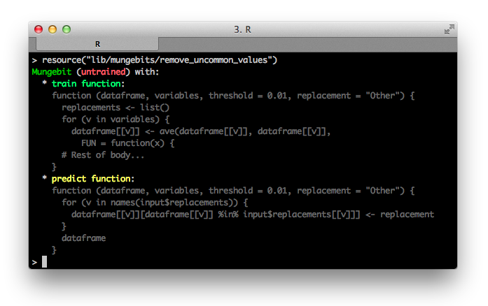
Let's see what happens when we run it on a simple example.
bit <- resource("lib/mungebits/remove_uncommon_values")
iris$Species <- as.character(iris$Species)
iris[1, "Species"] <- "Bumblebee"
head(bit$run(iris, "Species"), 2)
#   Sepal.Length Sepal.Width Petal.Length Petal.Width Species
# 1          5.1         3.5          1.4         0.2   Other
# 2          4.9           3          1.4         0.2  setosa
What happens when we run it on a single row of iris data?
bit$run(iris[1:2, ], "Species") # We never modified iris.
#   Sepal.Length Sepal.Width Petal.Length Petal.Width Species
# 1          5.1         3.5          1.4         0.2   Other
# 1          5.1         3.5          1.4         0.2   setosa
Our feature engineering step is now "production ready"! We can replay it on streaming rows of new data or on new validation sets to determine whether our classifier is behaving as expected.
bit$train(iris[1, ])
# Error:
#   This mungebit has already been trained, cannot re-train.
Training a mungebit is like flipping a one-time switch: once we do it, we can't undo it; we would need a new fresh mungebit. This way, we can be sure that once we have fed in our initial training set its specific characteristics will be used to replay the feature engineering example as it happened.
For example, if a rare
value was on the border of the 0.01 threshold then certain subsamples
of the training set might consider it rare and replaceable with
"Other" whilst different subsamples do not. If we didn't have mungebits, we would
need to write a separate data pipeline for each model as to be
very careful about these sorts of edge cases. Incorrectly failing
to replace a value could lead to bizarre bugs in our classifier
when the column gets converted to a categorical feature. Instead, the unified
bit$run(...) interface means the only
time we will ever have to think about the train versus predict
distinction is when we are writing our mungebit.
Testing Mungebits
Let's write some tests to convince ourselves our implementation is valid.
# test/lib/mungebits/remove_uncommon_values.R
test_that("it does not replace a common value", {
  bit <- resource()
  iris$Species <- as.character(iris$Species)
  # Test the mungebit when it is training.
  expect_equal(as.character(bit$run(iris, "Species")[1, 5]), "setosa")
  stopifnot(bit$trained())
  # And when it is predicting.
  expect_equal(as.character(bit$run(iris, "Species")[1, 5]), "setosa")
})
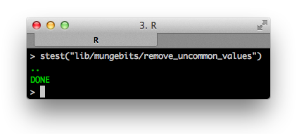
Looking pretty good! Note we used stest, a helper
provided by the Syberia modeling engine, to test our "resource", in this case the mungebit.
The point of good tests is to anticipate not only the example for which you wrote the code, but every possible input anyone could ever throw at it, so there are no surprises if someone uses your code in a way you did not expect.
# Continued: test/lib/mungebits/remove_uncommon_values.R
test_that("it replaces an uncommon value", {
  bit <- resource()
  iris$Species <- as.character(iris$Species)
  iris[1, 5] <- "Bumblebee"
  expect_equal(bit$run(iris, "Species")[1, 5], "Other")
  expect_equal(bit$run(iris, "Species")[1, 5], "Other")
})

test_that("it replaces a previously-unseen value", {
  bit <- resource()
  iris$Species <- as.character(iris$Species)
  iris[1, 5] <- "Bumblebee"
  expect_equal(bit$run(iris, "Species")[1, 5], "Other")
  iris[1, 5] <- "Flubber"
  expect_equal(bit$run(iris, "Species")[1, 5], "Other")
})
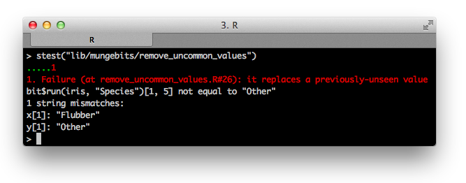
Oh no! Our first test failure. Writing tests is about stepping outside of the box of how you think about the work you have created and considering every possible scenario for how other people may use it. In this case, if we had encountered a new data point with a value that was not observed during the training process, we would have failed to replace it with "Other" — even though its incidence in the original data was 0%!
This is a very common oversight. While writing the original code, we assumed that we wish to replace values that are uncommon. We stored them for later so that we could repeat the same process when new data came in. However, we failed to take into account that future data could have an infinite number of possible values. We should have instead stored the very finite list (by the pigeonhole principle, at most 100) of common values: those with incidence more than 1%.
# lib/mungebits/remove_uncommon_values.R
train <- function(dataframe, variables, threshold = 0.01, replacement = "Other") {
  common_values <- list()
  for (v in variables) {
    dataframe[[v]] <- ave(dataframe[[v]], dataframe[[v]], FUN = function(x) {
      if (length(x) / NROW(dataframe) < threshold) {
        "Other"
      } else {
        common_values[[v]] <<- c(common_values[[v]], x[1L])
        x[1L]
      }
    })
  }
  # We'll learn about the "input" helper shown below later on.
  input$common_values <- common_values
  dataframe
}

predict <- function(dataframe, variables, threshold = 0.01, replacement = "Other") {
  variables <- intersect(colnames(dataframe), variables)
  for (v in names(input$common_values)) {
    dataframe[[v]][!is.element(dataframe[[v]], input$common_values[[v]])] <- replacement
  }
  dataframe
}
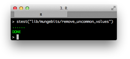
The more tests we write, the more coverage we have. You can think of test coverage (how much of your code is covered by test cases) as insurance on future changes to the code base. As the amount of code we write increases and the project becomes more complex, it will be harder and harder to track what everyone's assumptions are about the inputs and outputs to all the functions and resources used throughout the project. If someone ever fixes a bug or refactors anything, having lots of tests means it will be very easy to tell if they broke something in the process. At Avant we have used this approach to create data science collaboration repositories with tens of thousands of commits, thousands of models, and dozens of collaborators without stumbling on complexity: tests pay off.
Next Steps
Continue reading below for the more advanced and thorough mungebits section, or proceed with stagerunners if you'd like the abbreviated tour. You can always come back to finish the more advanced use cases.
Advanced mungebits
The purpose of mungebits is to give a syntax for rapidly cleaning data and experimenting with feature engineering without having to rewrite anything when it comes time to productionize. To write a data pipeline after having experimentally munged the data in the R console would be a wasted effort: the R munging should give you a data pipeline for free.
The primary abstractions provided by the mungebits2 package are:
Mungebit R6 class. A mungebit has the members
c("train_function", "predict_function", "input"), where the first two are both functions that take and return a dataframe (with possibly more parameters) and the last one is an environment object used by the train function to store metadata required by the predict function.Mungebits are meant to record the most abstract feature cleaning and engineering ideas: filter irrelevant columns, replace values, convert to a categorical, discretize, impute, apply PCA, etc. They are connected to a specific dataset through a mungepiece.
- Mungepiece R6 class. While a mungebit is the abstract data cleaning or feature engineering step, a mungepiece records the parameters passed to the mungebit as applied to a specific dataset.
- The munge function. Applying the munge function to a raw dataset and a list of untrained mungepieces will yield a trained list of mungepieces, a munge procedure, which can be applied to any future stream of the dataset drawn from the same distribution. For example, if someone gives you a validation set with three more months of data, or a new data record comes in through a streaming production system, the munge procedure will replay the feature engineering to clean up the data.
Although the Syberia modeling engine gives you a syntax for creating mungepieces to include in your data preparation, let's see what the process would look like when performed by hand.
We'll use Kaggle's Titanic data set.
data <- read.csv(stringsAsFactors = FALSE, "https://raw.githubusercontent.com/haven-jeon/introduction_to_most_usable_pkgs_in_project/master/bicdata/data/titanic.csv")
dim(data) # [1] 1309 15
home.dest representing
their home destination.
head(data$home.dest)
# [1] "St Louis, MO"                    "Montreal, PQ / Chesterville, ON"
# [3] "Montreal, PQ / Chesterville, ON" "Montreal, PQ / Chesterville, ON"
# [5] "Montreal, PQ / Chesterville, ON" "New York, NY"
extract_state <- function(strings) {
  has_state <- grepl("[A-Z]{2}", strings)
  output <- rep(NA_character_, length(strings))
  output[has_state] <- gsub(".*([A-Z]{2}).*", "\\1", strings[has_state])
  output
}
table(extract_state(data$home.dest))
# AB  BC  CA  CO  CT  DC  DE  FL  IA  IL  IN  KS  KY  MA  MB  ME  MI  MN  MO
# 2   4  12   3  13   6   1   1   4  26   3   4   2  28  12   3  21  20   4
# MT  ND  NE  NH  NI  NJ  NM  NS  NY  OH  ON  OR  PA  PQ  RI  SA  SD  UT  VA
#  4   4   1   1   1  34   1   2 145  24  20   6  28  18   5   2   3   1   3
# VT  WA  WI  WV
#  4   4   8   2
library(mungebits2) # devtools::install_github("syberia/mungebits2")
bit <- mungebit$new(function(dataframe, from, to) {
  extract_state <- function(strings) {
    has_state <- grepl("[A-Z]{2}", strings)
    output <- character(length(strings))
    output[has_state] <- gsub(".*([A-Z]{2}).*", "\\1", strings[has_state])
    output
  }
  dataframe[[to]] <- extract_state(dataframe[[from]])
  dataframe
})
# This call will set from = "home.dest" and to = "state".
states <- bit$run(data, "home.dest", "state")$state
stopifnot(identical(extract_state(data$home.dest), states)) # Passes.
We've already gained some clarity: we can re-use this mungebit for any dataset that has a character feature containing state as a substring and create a new feature representing that state.
In the modeling engine, the above would instead become one line of code in the model file with a separate file for the mungebit definition. This makes it clear the mungebit can be re-used on multiple datasets for a variety of purposes.
# One line of code in some models/dev/some_model.R
list(...,
  data = list(
    ...
  , "Parse out state" = list(extract_state, "home.dest", "state")
    ...
  )
)
# lib/mungebits/extract_state.R
# Note that the function "extract_state" in models/dev/some_model.R
# gets *injected*: we don't have to define it anywhere, since
# the modeling engine figures it out from the filename.
# We'll discuss the point of setting train = predict later.
train <- predict <- function(dataframe, from, to) {
  extract_state <- function(strings) {
    has_state <- grepl("[A-Z]{2}", strings)
    output <- character(length(strings))
    output[has_state] <- gsub(".*([A-Z]{2}).*", "\\1", strings[has_state])
    output
  }
  dataframe[[to]] <- extract_state(dataframe[[from]])
  dataframe
}
# test/lib/mungebits/extract_state.R
# Our test suite won't run without a test for the mungebit.
test_that("it can parse a simple state example", {
  data <- data.frame(location = c("Birmingham, AL", "Chicago, IL", "Mars"),
                     stringsAsFactors = FALSE)
  # resource() will build us the mungebit: same as mungebit$new(train)
  expect_equal(resource()$run(data, "location", "state")$state,
               c("AL", "IL", ""))
})
# Running stest("lib/mungebits/extract_state") should convince you
# the test suite passes.
This is a narrow transformation.
We can compute state on a passenger-by-passenger
basis. Narrow transformations are usually straightforward. This
is why we set train <- predict in the
mungebit definition. We are making it clear that we can use
the same code for cleaning the data offline versus running
it on new data. This is not always the case.
We stumble when we hit wide transformations,
where we must use information about other passengers to do the feature engineering step.
Different passengers will be on board the Titanic in different cabins and what cabin they're in (a good proxy for first class, second class, and third class) may be correlated with their state: passengers from one state may be on average more affluent than those in another and it may be unusual for a passenger from a certain state to be in a certain cabin. We can measure this by creating a feature that asks whether a passenger is in a cabin that the majority of the passengers from the state are in, i.e., does the passenger's cabin equal the mode (most frequently occuring value) of the cabins of the passengers in the same state?
head(data$cabin) # "B5" "C22 C26" "C22 C26" "C22 C26" "C22 C26" "E12"
# We probably need something less granular.
data$cabin_class <- gsub("[^A-Z]*", "", data$cabin) # "B" "C" "C" ...
string_mode <- function(x) {
  counts <- table(x)
  names(counts)[which.max(counts)]
} # string_mode(c("A", "A", "A", "B", "C")) = "A"
data$is_mode_of_cabin_class_by_state <- as.logical(
  ave(data$cabin_class, data$state, FUN = function(cabin_class) {
    # Mode doesn't make sense if everyone's in the same cabin
    # so for those values we set NA.
    if (length(unique(cabin_class)) == 1) { NA }
    # A lot of passenger's records don't have a cabin, so exclude those.
    else { cabin_class == string_mode(Filter(function(x) x != "", cabin_class)) }
  }))
table(data$is_mode_of_cabin_class_by_state) # FALSE - 1160, TRUE - 110
sum(is.na(data$is_mode_of_cabin_class_by_state)) # [1] 39
In practice, it may be very difficult to tell what will work and what won't work. We've certainly had our fair share of counter-intuitive variables that don't seem significant but, for example, may end up in many branches of a tree model. Comparing complex aggregations against concrete values is a good source of wide transformations and in many cases improves model performance. When in-the-flow trying out features like this, it is easy to forget how complex it may be to implement the features when new validation sets come along or streaming one-row data sets come through in production.
In the above example, the problem stems from the fact that we used
R's ave function. If we had fed different
subsamples of the dataset to the code, different feature engineering
could result depending on whether certain states have two top contenders
for most popular cabin! What if we want different models for different
groups of the passenger population? Should we use the cabin class mode of the
entire universe of passengers or restrict to each group? Both approaches
work, and the former is usually solved through ETL, while the latter
leads to a combinatorial explosion of data pipelines: we would need
to create a separate feature for each group of passengers we're
interested in modeling separately.
Not only that, but we won't be able to run the same code above when
a new data point comes in. We can't run ave
on a single row of data! We would need to remember the cabin class mode
for each state and then compare it against the state of the single row
when we stream (replay on one data point) the feature engineering step.
This is where mungebits shine. They allow you to unify your narrow and wide transformations, which together compose all transformations you could ever perform on any dataset in the universe, without introducing the technical debt that is typically associated with most ETL workflows. All of the feature engineering stays experimental, within the console, interactive, is replayable, and when it's all over with you have a very customized data pipeline for performing the same cleaning steps on a new row of data.
# models/dev/is_mode_in_group.R
# Generally, the data scientist will only need to play with this file.
list(...,
  data = list(
    ...
  , "Parse out state"       = list(extract_state, "home.dest", "state")
  # We'll cover multi_column_transformation later.
  , "Cabin class var"       = list(multi_column_transformation(gsub), "cabin", "cabin_class", pattern = "[^A-Z]*", replacement = "")
  , "Is pop cabin by state" = list(is_mode_in_group, "cabin_class", "state", exclude = c("", NA))
    ...
  )
)
# Move your mouse here -> x <- and scroll to the right.
# We take the one line per munge step approach and violate the
# typical column length developer sanity concern
# (lots of text on one row of a file is a nuisance to read and violates
# most style guides). This is so that when it gets too long, we can use
# our annoyance as a weapon to refactor the step into its own mungebit
# or condense the parametrization.
#
# It also makes it frictionless to comment out certain steps if you're
# experimenting and makes the full modeling procedure a joy to read.
# lib/mungebits/is_mode_in_group.R
# We're going to show you what a thorough implementation of this might
# look like. Feel free to breeze through this and come back to it when
# you feel fresh later.
variable_name <- function(target_variable, grouping_variable) {
  paste0("is_mode_of_", target_variable, "_by_", grouping_variable)
}

train <- function(data, target_variable, grouping_variable, name, exclude = NA_character_) {
  stopifnot(is.character(target_variable),
    is.character(grouping_variable), is.character(exclude),
    length(target_variable) == 1, length(grouping_variable) == 1,
    target_variable %in% colnames(data), grouping_variable %in% colnames(data))
  if (missing(name)) name <- variable_name(target_variable, grouping_variable)
  stopifnot(is.character(name) && length(name) == 1 && !is.na(name) && nzchar(name))

  if (!is.character(data[[target_variable]])) {
    stop("The is_mode_in_group mungebit currently only supports character features.")
  }

  string_mode <- function(x) {
    if (length(x) == 0) NA_character_
    else {
      counts <- table(x)
      names(counts)[which.max(counts)]
    }
  }

  input$modes <- list() # Store each mode by grouping variable.
  data[[name]] <- as.logical(
    ave(seq_len(NROW(data)), data[[grouping_variable]], FUN = function(ix) {
      var   <- data[ix, target_variable]
      group <- as.character(data[ix[1L], grouping_variable])
      if (length(unique(var)) == 1) {
        input$modes[[group]] <- NA
        NA
      } else {
        input$modes[[group]] <- mode <-
          string_mode(Filter(function(x) !x %in% exclude, var))
        ifelse(var %in% exclude, NA, var == mode)
      }
    })
  )
  data
}

predict <- function(data, target_variable, grouping_variable, name, exclude = NA_character_) {
  if (missing(name)) name <- variable_name(target_variable, grouping_variable)
  groups <- match(as.character(data[[grouping_variable]]), names(input$modes))
  var <- logical(NROW(data))
  var[is.na(groups)]  <- NA
  var[!is.na(groups)] <- as.logical(
    ave(seq_len(NROW(data)), data[[grouping_variable]], FUN = function(ix) {
      slice <- data[ix, target_variable]
      ifelse(slice %in% exclude, NA,
             slice == input$modes[[as.character(data[ix[1L], grouping_variable])]])
    }))
  data[[name]] <- var
  data
}
# test/lib/mungebits/is_mode_in_group.R
test_that("it can tell whether a target is in the mode of a group on a simple example", {
  data <- data.frame(stringsAsFactors = FALSE,
    target = c("A", "A", "A", "B", "C"), group = rep(1, 5))

  mb <- resource()
  expect_equal(
    mb$run(data, "target", "group")$is_mode_of_target_by_group,
    c(TRUE, TRUE, TRUE, FALSE, FALSE)
  )
  # Check that it works on one-row data as well.
  expect_true (mb$run(data[1, ], "target", "group")$is_mode_of_target_by_group)
  expect_false(mb$run(data[4, ], "target", "group")$is_mode_of_target_by_group)
})

test_that("it keeps track of different modes for different groups", {
  data <- data.frame(stringsAsFactors = FALSE,
    target = c("A", "A", "A", "B", "C", "C", "C", "C", "B", "A"),
    group = rep(c(1, 2), each = 5))

  mb <- resource()
  expect_equal(
    mb$run(data, "target", "group")$is_mode_of_target_by_group,
    c(TRUE, TRUE, TRUE, FALSE, FALSE, TRUE, TRUE, TRUE, FALSE, FALSE)
  )
  # Check that it works on one-row data as well.
  expect_true (mb$run(data[1, ], "target", "group")$is_mode_of_target_by_group)
  expect_false(mb$run(data[4, ], "target", "group")$is_mode_of_target_by_group)
  expect_true (mb$run(data[6, ], "target", "group")$is_mode_of_target_by_group)
  expect_false(mb$run(data[9, ], "target", "group")$is_mode_of_target_by_group)
})

test_that("it assigns NA to excluded labels", {
  data <- data.frame(stringsAsFactors = FALSE,
    target = c("A", "A", "A", "B", ""), group = rep(1, 5))
  mb <- resource()
  expect_equal(
    mb$run(data, "target", "group", exclude = "")$is_mode_of_target_by_group,
    c(TRUE, TRUE, TRUE, FALSE, NA)
  )
  # Check that it works on one-row data as well.
  expect_true (mb$run(data[1, ], "target", "group", exclude = "")$is_mode_of_target_by_group)
  expect_false(mb$run(data[4, ], "target", "group", exclude = "")$is_mode_of_target_by_group)
  expect_equal(mb$run(data[5, ], "target", "group", exclude = "")$is_mode_of_target_by_group, NA)
})
Wide transformations can be tricky to reproduce in future scenarios when new data comes in. By acknowleding this distinction and tackling the hidden complexity head-on through a convention with built-in testing, we can avoid headaches down the road when we find useful but difficult to procure features that will have to be replicated for future records.
By using mungebits—modular production-ready data preparation—you can stop wasting time cleaning data and get back to work on math and stats. If someone else finds a general feature engineering or data cleaning idea, and they have parametrized and tested it well, they can easily share it and you just have to plug in the parameters relevant to your data set.
Let's take a step back and look at a simpler wide transformation.
normalize <- function(variable, mean, stdev) {
  (variable - mean) / stdev
}

normalizer <- mungebit$new(function(data, variables) {
  input$means <- lapply(data[variables], mean, na.rm = TRUE)
  input$stdev <- lapply(data[variables], stats::sd, na.rm = TRUE)
  names(input$means) <- names(input$stdev) <- variables
  data[variables] <- Map(normalize, data[variables], input$means, input$stdev)
  data
}, function(data, variables) {
  # We should be careful since the variables may not be in the
  # same order when we're looking at new data.
  data[variables] <-
    Map(normalize, data[match(variables, names(input$means))],
        input$means, input$stdev)
  data
})

head(normalizer$run(iris, "Sepal.Length")$Sepal.Length)
# [1] -0.8976739 -1.1392005 -1.3807271 -1.5014904 -1.0184372 -0.5353840
head(normalizer$run(iris[1, ], "Sepal.Length")$Sepal.Length)
# [1] -0.8976739
We used the mungebit$new constructor to build
a new mungebit. The first argument is the train function, the
code that will be run the first time the run
method is called (i.e., during training) and has access to an environment
called input which will be stored on the
mungebit object and used during subsequent calls to run.
The second time we call that method it will execute the predict function,
the second argument that was passed to the normalizer.
You can think of the mungebit as a switch that, once flipped (trained), cannot be unflipped: it captures the essence of the feature engineering or data cleaning step and can be replayed on arbitrary subsets (including single rows or future single rows) of the same raw, messy data set.
Even normalizing your features is non-trivial to reproduce, in the sense that you have to be careful to recall the means and standard deviations to achieve the same normalization on single rows of data.
normalizer <- mungebit$new(column_transformation(function(variable) {
  if (!trained) {
    input$mean  <- mean(variable, na.rm = TRUE)
    input$stdev <- stats::sd(variable, na.rm = TRUE)
  } # column_transformation keeps track of the mean and standard
    # deviation of each column separately by "shadowing" the input helper.
  (variable - input$mean) / input$stdev
}))
# Running the above example will achieve the same results.
The column_transformation
helper function is exported by the mungebits2 library to deal with
a common type of operation: one that only touches one column.
For these column-shardable operations, you can restrict
your computation to each column individually and pass in the list
of columns to execute on later.
head(normalizer$run(iris, 1:4), 2) # Run the normalizer on the first four columns.
#   Sepal.Length Sepal.Width Petal.Length Petal.Width Species
# 1   -0.8976739  1.01560199    -1.335752   -1.311052  setosa
# 2   -1.1392005 -0.13153881    -1.335752   -1.311052  setosa
normalizer$run(iris[1, ], 1:4)
#   Sepal.Length Sepal.Width Petal.Length Petal.Width Species
# 1   -0.8976739    1.015602    -1.335752   -1.311052  setosa
You may also have noticed we didn't need a predict function
when defining the normalizer mungebit in the second format. The
trained helper logical is injected into any
mungebit train or predict function in case there is a large
amount of re-usable shared logic. Generally, if your code
for training and predicting varies by more than a few lines
you should split them up into two functions. Otherwise, you
can have a simple if (!trained) switch
to record the metadata you'll need in input
(e.g., means and standard deviations) to replay the munge step later.
